Blackbody Radiation and the Quantum Revolution
Introduction: A Tangled Dialogue Between Math and Physics
The study of blackbody radiation is one of the most striking cases in the history of science. It shows that mathematics is not merely a descriptive tool but a critical lens capable of challenging physical theories. By the late 19th century, it was a formula that “screamed”: something wasn’t adding up. Classical physics predicted an absurd outcome — infinite energy — and mathematics hinted at the need for a conceptual leap: quantization.
Science, in this sense, advances not only by observing the world but also by observing its own equations. The case of blackbody radiation highlights the deep interconnection between mathematics and physics — no hierarchy, just a continuous dialogue where abstraction guides, challenges, and sharpens physical understanding.
Radiation and Early Empirical Observations
When a body is heated, internal electric dipole vibrations emit electromagnetic radiation. As early as the late 1700s, it was observed that during porcelain firing, different materials glowed red at the same temperature, regardless of their chemical composition.
By the mid-1800s, spectroscopic studies revealed:
- Hot solids or liquids emit a continuous spectrum.
- Hot rarefied gases emit line spectra.
🔍 A spectrum is a body’s “light signature.” Solids glow across all frequencies, like glowing metal, while gases emit only specific ones, like neon lights.
Imagine an orchestra playing a warm tone. Some instruments emit low notes, corresponding to low frequencies, while others emit high notes, corresponding to high frequencies. The total sound is complex — just like the radiation from a hot body, composed of multiple frequencies, each carrying a certain amount of energy.
Energy distribution indicates how much energy exists at each frequency:
- At low temperature, most energy lies in the infrared region.
- At higher temperatures, visible frequencies — red, yellow, and eventually white — also gain intensity.
Energy Density and Spectral Distribution
We define the energy density per unit volume as
\[u(\vec{r}) = \frac{d\varepsilon}{d\tau} \qquad \left[ \frac{\mathrm{J}}{\mathrm{m}^3} \right]\]where r⃗ is the spatial position. The function u(r⃗) tells us how much energy is contained in a specific region of the cavity.
The spectral energy density is
\[\rho(\nu) = \frac{du}{d\nu} \qquad \left[ \frac{\mathrm{J}} {\mathrm{m}^3\cdot\mathrm{Hz}} \right]\]Thus, the energy between frequencies ν and ν + dν is
\[du = \rho(\nu)\,d\nu\]Integrating over all frequencies gives the total energy per unit volume:
\[u = \int_0^{+\infty} \rho(\nu)\,d\nu\]🔍 The function ρ(ν) shows how energy is distributed across frequencies. The larger ρ(ν) is, the greater the energy density associated with that frequency.
🔹 Think of the spectrum as a bar chart: each bar represents a frequency, and its height represents the corresponding energy density. The function ρ(ν) is the continuous curve describing this distribution.
Kirchhoff and the Ideal Blackbody
A blackbody, theorized by Gustav Kirchhoff in 1859, is an ideal object that absorbs all incoming electromagnetic radiation — no reflection and no transmission. Thermodynamic equilibrium implies a universal relation between absorption and emission.
Kirchhoff showed that, in thermal equilibrium, the ratio between emitted and absorbed power at a given frequency depends only on frequency and temperature. This function is universal: it applies to all blackbodies, regardless of shape or material.
🔍 If an object absorbs well at a certain frequency, it must also be an efficient emitter at that frequency. Otherwise, one could construct a process incompatible with thermal equilibrium and the second law of thermodynamics.
To physically model this, Kirchhoff imagined a cavity with walls and a tiny hole. A ray of light entering the hole undergoes repeated reflections and is overwhelmingly likely to be absorbed. Radiation escaping from the hole therefore provides an approximation to ideal blackbody radiation.
\[\frac{E_\nu}{A_\nu} = J(\nu,T)\]Blackbody Spectrum and Wavelength
Besides frequency ν, the spectrum can also be described in terms of wavelength λ.
The two quantities are related by
\[\nu = \frac{c}{\lambda}\]The spectral distribution may therefore also be expressed as a function of wavelength:
\[du = \rho(\lambda)\,d\lambda\]🔍 It is often more intuitive to use wavelength: red light is around 700 nm, while blue light is around 450 nm.
The graph of the spectral distribution as a function of wavelength has a characteristic maximum, and the position of this maximum shifts toward shorter wavelengths as temperature increases.
📌 This peak is described by Wien’s displacement law.
Wien’s Law and Total Emitted Energy
In 1893, Wien proposed a spectral form of the type
\[\rho(\nu) = \nu^3 F\left(\frac{\nu}{T}\right)\]This means that the temperature dependence enters through the ratio ν/T.
🔍 Changing the temperature shifts and rescales the spectrum according to a universal structure.
Integrating the spectral energy density over all frequencies gives a total energy density proportional to the fourth power of temperature:
\[u \propto T^4\]The corresponding law for the total radiant exitance of a blackbody is the Stefan–Boltzmann law:
\[M = \sigma T^4\]where σ is the Stefan–Boltzmann constant.
📌 The total emitted radiant power per unit area grows with the fourth power of absolute temperature.
Wien’s Displacement Law
The position of the maximum of the wavelength spectrum satisfies
\[\frac{d\rho_\lambda}{d\lambda} = 0\]and leads to Wien’s displacement law:
\[\lambda_{\mathrm{max}}T = b\]where b is Wien’s displacement constant.
📌 The hotter a body becomes, the shorter the wavelength at which its emission spectrum reaches its maximum. This helps explain the progression from red to increasingly white light in heated objects.
Classical Prediction: Rayleigh–Jeans Law
Under classical assumptions, the spectral energy density is
\[\rho(\nu) = \frac{8\pi\nu^2kT}{c^3}\]📌 This expression works well at low frequencies but diverges as the frequency tends to infinity:
\[\nu\to+\infty\]The resulting divergence became known as the ultraviolet catastrophe.
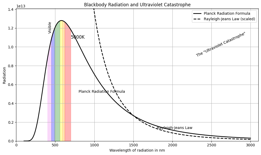
📊 The graph shows how the classical Rayleigh–Jeans prediction grows without bound at high frequencies, while Planck’s quantum model reproduces the observed spectrum.
Oscillators and Planck’s Insight
🔍 Why oscillators?
To model the interaction between matter and electromagnetic radiation, Planck considered microscopic oscillators associated with the cavity walls that could exchange energy with the electromagnetic field.
These were not intended as literal mechanical springs. They formed part of a theoretical model connecting characteristic frequencies with the exchange of energy.
The oscillator model allowed Planck to investigate the statistical distribution of energy associated with radiation at different frequencies.
Planck’s Solution
In 1900, Planck introduced the hypothesis that the energy associated with oscillators of frequency ν could take discrete values:
\[E_n = nh\nu\]with
\[n = 0,1,2,\dots\]Here h is Planck’s constant and ν is the oscillator frequency.
📌 In Planck’s original formulation, the energy of the oscillators was quantized. The stronger interpretation of electromagnetic radiation itself as consisting of light quanta would be developed later.
Using statistical arguments, Planck obtained the spectral energy density
\[\rho(\nu) = \frac{8\pi h\nu^3}{c^3} \frac{1} {e^{h\nu/(kT)}-1}\]This expression reproduces the appropriate limiting behavior:
\[h\nu\ll kT\]gives the Rayleigh–Jeans regime, while
\[h\nu\gg kT\]gives the Wien regime.
Planck’s constant has the value
\[h \approx 6.62607015\times10^{-34} \ \mathrm{J\,s}\]📌 The introduction of h and discrete energy elements marked one of the decisive beginnings of quantum theory.
Final Reflection: Math, Physics, and Paradigm Shifts
Blackbody radiation reveals the essential role of mathematics in science. Classical theory, supported by principles such as energy equipartition, seemed extraordinarily successful — until its predictions conflicted with the observed spectrum.
📌 Here, mathematics does not merely describe: it exposes a structural incompatibility between a theoretical framework and physical observation.
Planck’s quantum hypothesis provided the mathematical structure capable of reproducing the blackbody spectrum. Its significance eventually extended far beyond the original radiation problem and contributed to the emergence of quantum theory.
🔍 The blackbody crisis shows how scientific theories, though coherent and powerful within their domains, can encounter limits. When those limits become experimentally unavoidable, new concepts and new mathematical structures may be required.
Appendix: Mathematical Derivation of Planck’s Law
Planck assumed discrete energy levels:
\[E_n = nh\nu\]with
\[n = 0,1,2,\dots\]Using the Boltzmann factor, the average energy is
\[\bar{E} = \frac{ \displaystyle \sum_{n=0}^{\infty} nh\nu\, e^{-nh\nu/(kT)} }{ \displaystyle \sum_{n=0}^{\infty} e^{-nh\nu/(kT)} }\]Evaluating the geometric sums gives
\[\bar{E} = \frac{h\nu} {e^{h\nu/(kT)}-1}\]The number of electromagnetic modes per unit volume in the frequency interval from ν to ν + dν is
\[dN = \frac{8\pi\nu^2}{c^3} \,d\nu\]Multiplying the density of modes by the average energy per mode gives Planck’s spectral energy density:
\[\rho(\nu) = \frac{8\pi\nu^2}{c^3} \bar{E}\]Therefore,
\[\rho(\nu) = \frac{8\pi h\nu^3}{c^3} \frac{1} {e^{h\nu/(kT)}-1}\]Classical Limits
For high frequencies,
\[h\nu \gg kT\]and therefore
\[e^{h\nu/(kT)} \gg 1\]so
\[\frac{1} {e^{h\nu/(kT)}-1} \approx e^{-h\nu/(kT)}\]Hence,
\[\rho(\nu) \approx \frac{8\pi h\nu^3}{c^3} e^{-h\nu/(kT)}\]which gives the Wien high-frequency limit.
For low frequencies,
\[h\nu \ll kT\]we use
\[e^{h\nu/(kT)} \approx 1+\frac{h\nu}{kT}\]Therefore,
\[\frac{1} {e^{h\nu/(kT)}-1} \approx \frac{kT}{h\nu}\]and Planck’s law becomes
\[\rho(\nu) \approx \frac{8\pi\nu^2kT}{c^3}\]which is the Rayleigh–Jeans law.